Comparison of classifiers’ robustness to label noise
Viktor Petukhov
2018-02-01
Source file: notebooks/low_quality_cells/label_noise_robustness.Rmd
Last updated: 2018-02-02
Code version: b8b2fd2
Initialization
library(ggplot2)
library(ggrastr)
library(parallel)
library(dplyr)
library(dropestr)
library(dropEstAnalysis)
library(reshape2)
library(randomForest)
library(ggpubr)
library(cowplot)

theme_set(theme_base)

RgpPredict <- function(clf, x) {
  predictions <- predictORMCGP(clf, x)$prob[,2]
  names(predictions) <- rownames(x)
  return(predictions)
}

classifier_funcs <- list(
  KDE=list(train=TrainKDE, predict=function(clf, y) PredictKDE(clf, y)[, 2]),
  RF=list(train=function(x, y) randomForest(x=x, y=as.factor(y), ntree=1000, mtry=2),
          predict=function(clf, x) predict(clf, x, type='prob')[,2]),
  RGP=list(train=function(x, y) epORGPC(x, as.factor(y), kernel='gaussian'),
           predict=RgpPredict))
kPlotDir <- '../../output/figures/'
holder <- readRDS('../../data/dropest/allon_new/SRR3879617/est_11_22/cell.counts.rds')
holder$reads_per_umi_per_cell <- NULLNumber of cells:
analised_cbs <- names(sort(holder$aligned_umis_per_cell, decreasing=T)[1:1300])
umi_counts <- holder$aligned_umis_per_cell[analised_cbs]

features <- PrepareLqCellsDataPipeline(holder, mit.chromosome.name="chrM")[analised_cbs,]
classifier_data <- GetOptimalPcs(features)$pca.data
cell_number <- EstimateCellsNumber(umi_counts)

real_cbs <- analised_cbs[1:cell_number$min]
background_cbs <- analised_cbs[cell_number$max:length(analised_cbs)]

scores_base <- mclapply(classifier_funcs, ScoringFunction, classifier_data,
                        real_cbs, background_cbs, mc.cores=3)

PlotCellsNumberLine(umi_counts, estimate.cells.number=T, breaks=50) +
  theme_pdf()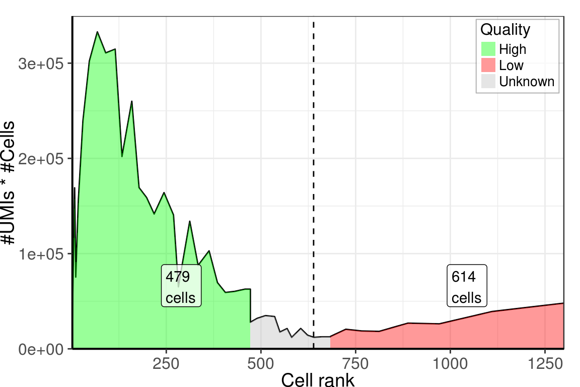
Miochondrial fraction:
smoothScatter(features$MitochondrionFraction, xlab='Cell rank',
              ylab='Mitochondrion fraction', cex.lab=1.2)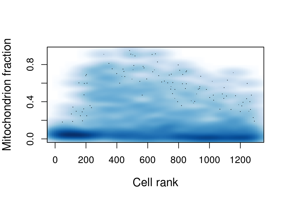
CV on labeled data
Simple cross-validation on labeled data. While, labels have errors, it can give us an estimate of the algorithms’ quality.
kfold_labeled_res <- lapply(classifier_funcs, function(clf)
  KFoldCV(classifier_data[c(real_cbs, background_cbs),],
          c(rep(1, length(real_cbs)), rep(0, length(background_cbs))),
          clf$train, clf$predict, k=5, stratify=F,
          measure = c('sensitivity', 'specifisity')))

CvResultsTable(kfold_labeled_res)| Classifier | sensitivity | specifisity |
|---|---|---|
| KDE | 90 (±4) | 90.7 (±1.2) |
| RF | 89.1 (±3.8) | 91.9 (±1) |
| RGP | 87.7 (±2.3) | 95.1 (±1.9) |
Stability of labels on CV
Let’s check robustness to data subsetting. Now we will remove 20% of train data, but check unswers on the same dataset (with “Unknown” quality). Here, “correct” answer is the answer, obtained after training on the whole dataset.
train_cbs <- c(real_cbs, background_cbs)
intermediate_cbs <- setdiff(analised_cbs, train_cbs)

intermediate_res <- mapply(function(scores, clf)
  KFoldCV(classifier_data[train_cbs,], scores[train_cbs], clf$train, clf$predict,
          k = 5, stratify = F, test.force = list(x=classifier_data[intermediate_cbs,],
                                                 y=scores[intermediate_cbs]),
          measure = c('sensitivity', 'specifisity')),
  scores_base, classifier_funcs, SIMPLIFY=F) %>%
  setNames(names(classifier_funcs))

CvResultsTable(intermediate_res)| Classifier | sensitivity | specifisity |
|---|---|---|
| KDE | 90.2 (±4.1) | 96.3 (±0.6) |
| RF | 89.8 (±6.1) | 96.5 (±1.9) |
| RGP | 83.5 (±2.6) | 99.3 (±0.6) |
Dependency between scores and borders
Again, we will check stability on “Unknown” cells. But now, we will widen borders of real / background cells. To estimate confidence intervals we randomly removes 10% of data (as in 10-fold CV).
offset_vals <- seq(0.0, 0.95, 0.05)
offset_accs <- mclapply(names(classifier_funcs), function(n)
  mclapply(offset_vals, function(offset)
    ScoreDependsOnBorders(classifier_data, scores_base[[n]], classifier_funcs[[n]],
                          real_cbs, background_cbs, offset, offset), mc.cores=20), mc.cores=2)
names(offset_accs) <- names(classifier_funcs)
plot_df <- lapply(offset_accs, function(df) lapply(1:length(offset_vals), function(i)
cbind(df[[i]], Measure=rownames(df[[i]]), Offset=offset_vals[i])) %>% bind_rows()) %>%
bind_rows(.id="Classifier") %>% mutate(mean=1-mean)
plot_df$Measure <- c('False negative rate', 'False positive rate')[as.integer(plot_df$Measure)]
gg_borders <- ggplot(plot_df, aes(x=Offset, ymin=mean-sd, ymax=mean+sd,
y=mean, color=Classifier, shape=Measure)) +
geom_pointrange(fatten=2.5, alpha=0.8, size=0.8) +
geom_line(aes(linetype=Measure), size=0.8, alpha=0.7) +
xlim(0, 1) +
scale_color_manual(values = c("#4E58E0", "#F08000", "#349147")) +
labs(x='Border offset', y='Value') +
theme_pdf()
gg_borders
Robustness to errors in labels
Let’s assume that classifier answers are real class labels. We will introduce some noise to them and retrain the classifiers on the noisy labels. Here, 75% of the dataset are used to train classifiers, and 25% are used to test them.
Symmetric errors
wrong_frac_vals <- seq(0.0, 1.0, 0.1)

var_types <- c('fpr', 'fnr')
wrong_labels_vars <- list(wrong=paste0('wrong.', var_types), all=paste0('all.', var_types), test=paste0('test.', var_types))

scores_with_err <- mcmapply(function(clf, scores)
  mclapply(wrong_frac_vals, function(frac) mclapply(1:10, function(y)
      ScoreCellsWithWrongLabels(classifier_data, scores, clf, frac, frac, 0.25), mc.cores=2), mc.cores=10),
  classifier_funcs, scores_base, SIMPLIFY=F, mc.cores=2)

names(scores_with_err) <- names(classifier_funcs)
Test data
Results on the test subset (25% of data):
measure_names <- c(fpr='False positive rate', fnr='False negative rate')
gg_offset_test <- scores_with_err %>%
  PlotTestedClassifierErrors(wrong_frac_vals, wrong_labels_vars, var_types,
                             filt.subset='test', measure.names=measure_names) +
  theme_pdf()

gg_offset_test
Changed labels
Results on cells with changed labels:
gg_offset_wrong <- scores_with_err %>%
  PlotTestedClassifierErrors(wrong_frac_vals, wrong_labels_vars, var_types,
                             filt.subset='wrong', measure.names=measure_names) +
  theme_pdf()

gg_offset_wrong
Nonsymmetric errors
Errors in real CBs only:
wrong_frac_vals_one_side <- wrong_frac_vals[1:(length(wrong_frac_vals) - 1)]

scores_with_err_real <- mcmapply(function(clf, scores)
  mclapply(wrong_frac_vals, function(frac) mclapply(1:10, function(y)
      ScoreCellsWithWrongLabels(classifier_data, scores, clf, frac, 0.0, 0.25), mc.cores=2),
      mc.cores=10),
  classifier_funcs, scores_base, SIMPLIFY=F, mc.cores=2)

PlotTestedClassifierErrors(scores_with_err_real, wrong_frac_vals_one_side,
                           wrong_labels_vars, var_types) +
  theme_pdf(legend.pos=c(0, 1))
Errors in background CBs only:
scores_with_err_background <- mcmapply(function(clf, scores)
  mclapply(wrong_frac_vals, function(frac) mclapply(1:10, function(y)
      ScoreCellsWithWrongLabels(classifier_data, scores, clf, 0.0, frac, 0.25), mc.cores=2),
      mc.cores=10),
  classifier_funcs, scores_base, SIMPLIFY=F, mc.cores=2)

PlotTestedClassifierErrors(scores_with_err_background, wrong_frac_vals_one_side,
                           wrong_labels_vars, var_types) +
  theme_pdf(legend.pos=c(0, 1))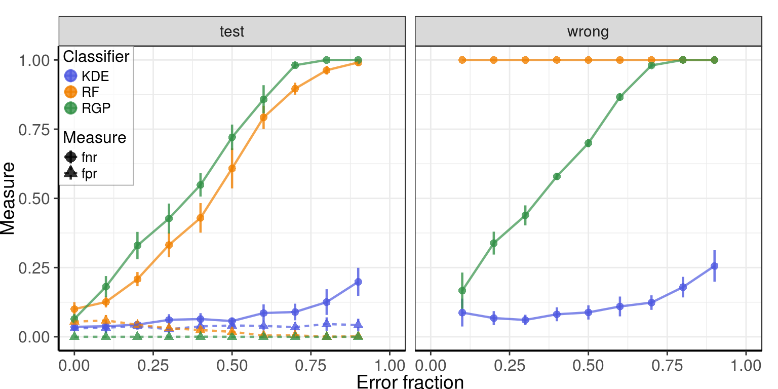
Complete figure
plotlist <- list(gg_offset_test, gg_offset_wrong, gg_borders) %>%
  lapply(function(gg) gg + rremove("legend")) %>%
  lapply(`+`, theme(plot.margin=ggplot2::margin()))

legend <- get_legend(
  gg_borders +
    scale_color_manual(values = c("#4E58E0", "#F08000", "#349147"),
                       labels=c("Kernel density estimation", "Random forest",
                                "Robust Gaussian processes")) +
    guides(color=guide_legend(override.aes=list(size=0.25)),
           shape=guide_legend(override.aes=list(size=0.5))) +
    theme(legend.box.background=element_blank(),
          legend.text=element_text(size=11),
          legend.title=element_text(size=13)))

plotlist[[1]] <- plotlist[[1]] + rremove("x.text") + rremove("x.ticks") + rremove("xlab")
plotlist[[3]] <- plotlist[[3]] + rremove("y.text") + rremove("y.ticks") + rremove("ylab")

gg_figure <- plot_grid(plotlist[[1]], legend, plotlist[[2]], plotlist[[3]], ncol=2,
                       rel_widths=c(1, 0.9), rel_heights=c(0.9, 1),
                       labels=c('A', '', 'B', 'C'), label_y=0.98,
                       label_x=c(0.15, 0.0, 0.15, 0.02)) +
  theme(plot.margin=ggplot2::margin(2, 2, 2, 2))

ggsave(paste0(kPlotDir, 'supp_label_noise_robustness.pdf'),
       gg_figure, width=8, height=6)
gg_figure
Session information
| value | |
|---|---|
| version | R version 3.4.1 (2017-06-30) |
| os | Ubuntu 14.04.5 LTS |
| system | x86_64, linux-gnu |
| ui | X11 |
| language | (EN) |
| collate | en_US.UTF-8 |
| tz | America/New_York |
| date | 2018-02-02 |
| package | loadedversion | date | source | |
|---|---|---|---|---|
| 1 | assertthat | 0.2.0 | 2017-04-11 | CRAN (R 3.4.1) |
| 2 | backports | 1.1.2 | 2017-12-13 | cran (@1.1.2) |
| 4 | bindr | 0.1 | 2016-11-13 | CRAN (R 3.4.1) |
| 5 | bindrcpp | 0.2 | 2017-06-17 | CRAN (R 3.4.1) |
| 6 | clisymbols | 1.2.0 | 2017-05-21 | cran (@1.2.0) |
| 7 | colorspace | 1.2-6 | 2015-03-11 | CRAN (R 3.3.1) |
| 9 | cowplot | 0.8.0 | 2017-07-30 | CRAN (R 3.4.1) |
| 11 | digest | 0.6.15 | 2018-01-28 | cran (@0.6.15) |
| 12 | dplyr | 0.7.4 | 2017-09-28 | cran (@0.7.4) |
| 13 | dropEstAnalysis | 0.6.0 | 2018-02-02 | local (VPetukhov/dropEstAnalysis@NA) |
| 14 | dropestr | 0.7.5 | 2018-02-01 | local (@0.7.5) |
| 15 | evaluate | 0.10.1 | 2017-06-24 | cran (@0.10.1) |
| 16 | ggplot2 | 2.2.1 | 2016-12-30 | cran (@2.2.1) |
| 17 | ggpubr | 0.1.4 | 2017-06-28 | CRAN (R 3.4.1) |
| 18 | ggrastr | 0.1.5 | 2018-01-29 | Github (VPetukhov/ggrastr@cc56b45) |
| 19 | git2r | 0.21.0 | 2018-01-04 | cran (@0.21.0) |
| 20 | glue | 1.2.0 | 2017-10-29 | cran (@1.2.0) |
| 24 | gtable | 0.2.0 | 2016-02-26 | CRAN (R 3.3.1) |
| 25 | highr | 0.6 | 2016-05-09 | CRAN (R 3.3.1) |
| 26 | htmltools | 0.3.6 | 2017-04-28 | cran (@0.3.6) |
| 27 | KernSmooth | 2.23-15 | 2015-06-29 | CRAN (R 3.4.0) |
| 28 | knitr | 1.19 | 2018-01-29 | cran (@1.19) |
| 29 | ks | 1.11.0 | 2018-01-16 | cran (@1.11.0) |
| 30 | labeling | 0.3 | 2014-08-23 | CRAN (R 3.3.1) |
| 31 | lattice | 0.20-35 | 2017-03-25 | CRAN (R 3.3.3) |
| 32 | lazyeval | 0.2.0 | 2016-06-12 | cran (@0.2.0) |
| 33 | magrittr | 1.5 | 2014-11-22 | CRAN (R 3.3.1) |
| 34 | Matrix | 1.2-10 | 2017-04-28 | CRAN (R 3.4.0) |
| 35 | mclust | 5.4 | 2017-11-22 | cran (@5.4) |
| 37 | munsell | 0.4.3 | 2016-02-13 | CRAN (R 3.3.1) |
| 38 | mvtnorm | 1.0-7 | 2018-01-26 | cran (@1.0-7) |
| 40 | pcaPP | 1.9-73 | 2018-01-14 | CRAN (R 3.4.1) |
| 41 | pillar | 1.1.0 | 2018-01-14 | cran (@1.1.0) |
| 42 | pkgconfig | 2.0.1 | 2017-03-21 | cran (@2.0.1) |
| 43 | plyr | 1.8.4 | 2016-06-08 | CRAN (R 3.3.1) |
| 44 | R6 | 2.2.2 | 2017-06-17 | cran (@2.2.2) |
| 45 | randomForest | 4.6-12 | 2015-10-07 | CRAN (R 3.4.1) |
| 46 | Rcpp | 0.12.15 | 2018-01-20 | cran (@0.12.15) |
| 47 | reshape2 | 1.4.2 | 2016-10-22 | cran (@1.4.2) |
| 48 | rlang | 0.1.6 | 2017-12-21 | cran (@0.1.6) |
| 49 | rmarkdown | 1.8 | 2017-11-17 | cran (@1.8) |
| 50 | rprojroot | 1.3-2 | 2018-01-03 | cran (@1.3-2) |
| 51 | scales | 0.4.1 | 2016-11-09 | cran (@0.4.1) |
| 52 | sessioninfo | 1.0.0 | 2017-06-21 | cran (@1.0.0) |
| 54 | stringi | 1.1.1 | 2016-05-27 | CRAN (R 3.3.1) |
| 55 | stringr | 1.2.0 | 2017-02-18 | CRAN (R 3.4.1) |
| 56 | tibble | 1.4.2 | 2018-01-22 | cran (@1.4.2) |
| 59 | withr | 2.1.1 | 2017-12-19 | cran (@2.1.1) |
| 60 | yaml | 2.1.16 | 2017-12-12 | cran (@2.1.16) |
This R Markdown site was created with workflowr