Drop-seq human/mouse mixture analysis
Viktor Petukhov
2018-01-23
Source file: notebooks/human_mouse/hm_drop_seq.Rmd
Last updated: 2018-02-04
Code version: 0306e1c
library(ggplot2)
library(ggrastr)
library(dplyr)
library(dropestr)
library(dropEstAnalysis)
library(Matrix)

theme_set(theme_base)
Load data
Here bam file was filtered by realigning it with kallisto 0.43 separately on mouse and human genome. Only reads, which were aligned only on one of them were used in dropEst.
# holder <- readRDS('../../data/dropest/dropseq/thousand/est_2018_01_26_tophat/thousand.rds')
# saveRDS(holder$cm_raw, '../../data/dropest/dropseq/thousand/est_2018_01_26_tophat/cm.rds')
cm <- readRDS('../../data/dropest/dropseq/thousand/est_2018_01_26_tophat/cm.rds')
kPlotDir <- '../../output/figures/'
cell_number <- 1100
gene_species <- ifelse(substr(rownames(cm), 1, 2) == "HU", 'Human', 'Mouse') %>%
as.factor()
umi_by_species <- lapply(levels(gene_species), function(l) cm[gene_species == l,] %>%
Matrix::colSums()) %>% as.data.frame() %>%
`colnames<-`(levels(gene_species)) %>% tibble::rownames_to_column('CB') %>%
as_tibble() %>%
mutate(Total = Human + Mouse, Organism=ifelse(Human > Mouse, "Human", "Mouse"),
IsReal=rank(Total) >= length(Total) - cell_number) %>%
filter(Total > 20)
mit_genes <- rownames(cm)[grep("_MT:.+", rownames(cm))]
umi_by_species$MitochondrionFraction <- GetGenesetFraction(cm, mit_genes)[umi_by_species$CB]
umi_by_species$Type <- ifelse(umi_by_species$IsReal, umi_by_species$Organism, "Background")
umi_by_species$Type[umi_by_species$Mouse > 5e3 & umi_by_species$Human > 5e3] <- 'Dublets'Common view
gg_template <- ggplot(umi_by_species, aes(x=Mouse, y=Human)) +
  geom_abline(aes(slope=1, intercept=0), linetype='dashed', alpha=0.5) +
  scale_x_log10(limits=c(1, 2e5), name="#Mouse molecules") +
  scale_y_log10(name="#Human molecules") + annotation_logticks() +
  theme_pdf(legend.pos=c(0.97, 0.05)) + theme(legend.margin=margin(l=3, r=3, unit="pt"))

gg_left <- gg_template +
  geom_point(aes(color=IsReal), size=0.1, alpha=0.15) +
  guides(color=guide_legend(override.aes=list(size=1.5, alpha=1)))

gg_right <- gg_template +
  geom_point(aes(color=MitochondrionFraction), size=0.1, alpha=0.15) +
  scale_color_gradientn(colours=c("#1200ba", "#347fff", "#cc4000", "#ff3333"),
                        values=scales::rescale(c(0, 0.1, 0.3, 0.8))) +
  guides(color=guide_colorbar(direction="horizontal", title.position="top",
                              title="Mitochondrial\nfraction",
                              barwidth=unit(1.0, units="in")))

cowplot::plot_grid(gg_left, gg_right)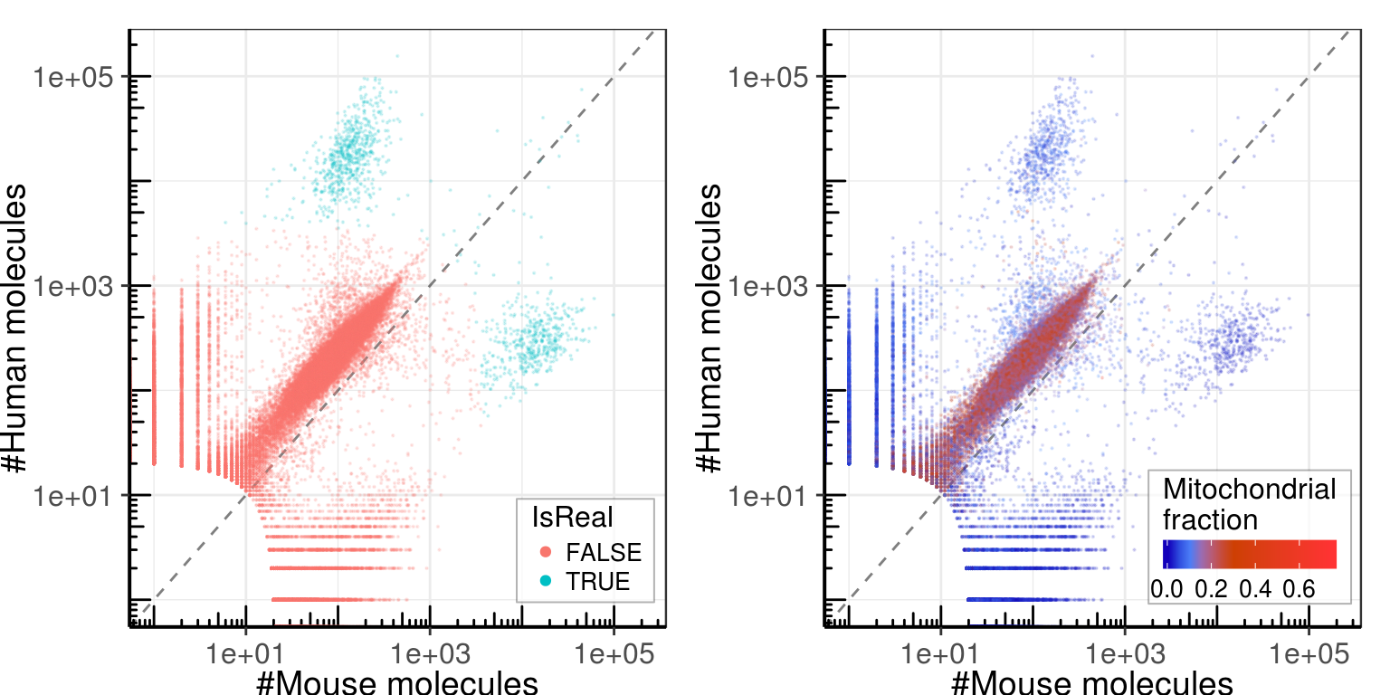
ggplot(umi_by_species) +
  geom_point(aes(x=Total, y=pmin(Human, Mouse) / Total, color=Organism), size=0.1,
             alpha=0.1) +
  scale_x_log10(name='#Real UMIs', limits=c(10, 2e5)) + annotation_logticks() +
  ylab('Fraction of mixed UMIs') +
  guides(color=guide_legend(override.aes=list(size=1.5, alpha=1))) +
  theme_pdf(legend.pos=c(1, 1))
Check for constant background
Background cells have constant fraction of mouse and human reads. Though this fraction is not determined by the corresponding ratio in real cells:
mouse_frac <- umi_by_species %>% filter(IsReal) %>%
  summarise(Mouse=sum(Mouse[Organism == 'Mouse']), Human=sum(Human[Organism == 'Human']),
            MF=Mouse / (Mouse + Human)) %>% .$MF

ggplot(umi_by_species) +
  geom_histogram(aes(x=Mouse / Total, y=..density.., fill=IsReal), binwidth=0.005, position="identity") +
  geom_vline(xintercept=mouse_frac) +
  xlab("Fraction of mouse reads") +
  theme_pdf(legend.pos=c(1, 1))
Distribution of total number of molecules by background cells:
gg <- ggplot(umi_by_species %>% filter(!IsReal)) +
  geom_histogram(aes(x=Total), bins=100) +
  scale_x_continuous(limits=c(0, 1000), expand=c(0, 0), name="Total #UMIs") +
  scale_y_continuous(limits=c(0,4500), expand=c(0, 0), name="#Cells") +
  theme_pdf()

gg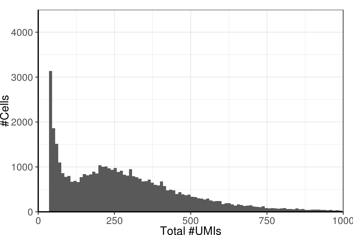
Though, it looks better on logscale:
gg +
  scale_x_log10(limits=c(19, 3000), expand=c(0, 0), name="Total #UMIs") +
  annotation_logticks(sides="b")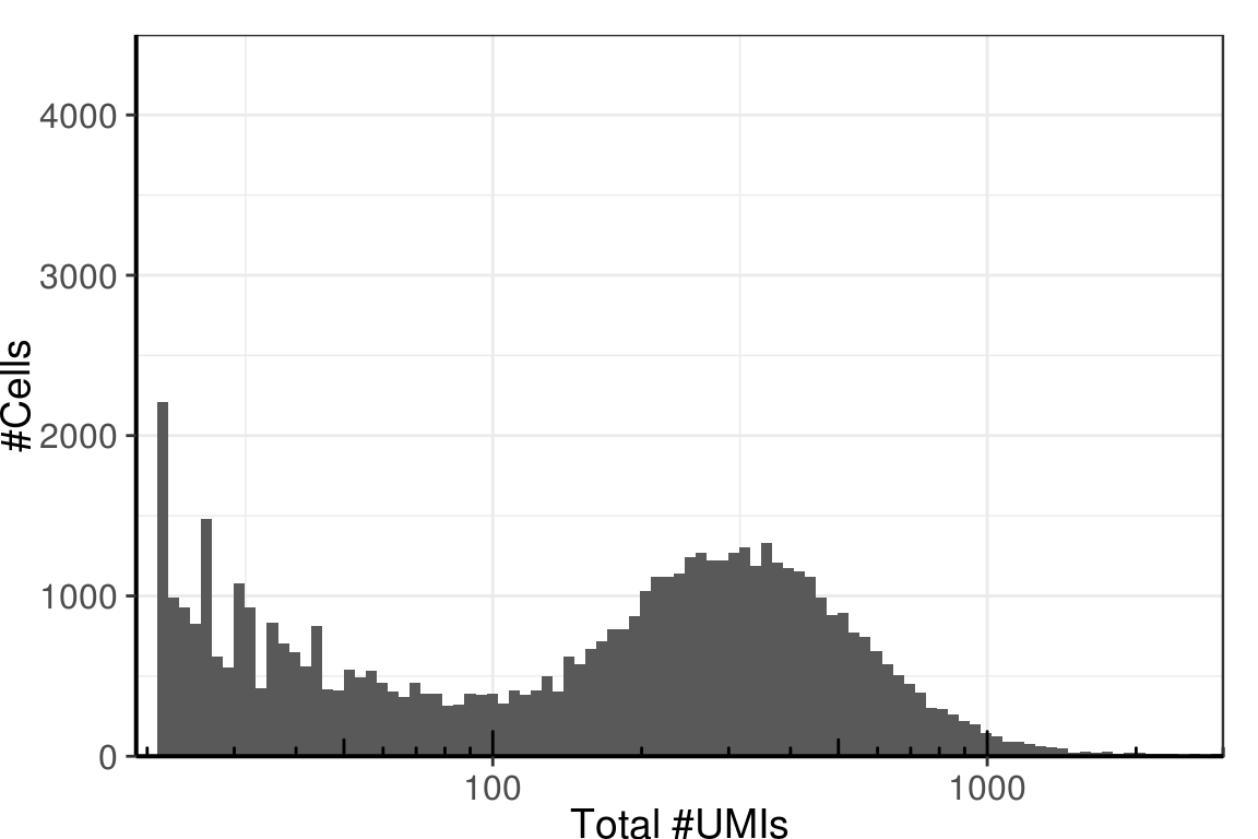
Figure
arrows_df <- umi_by_species %>% group_by(Type) %>%
  summarise(MouseEnd=median(Mouse), HumanEnd=median(Human)) %>%
  mutate(Mouse=c(1e1, 6e4, 2e1, 6e4),
         Human=c(1e3, 5e3, 7e4, 7e1))

fig_width <- 3.7
fig_height <- 4.4

gg_fig <- gg_template +
  geom_point_rast(aes(color=MitochondrionFraction), size=0.2, alpha=0.15,
                  width=fig_width, height=fig_height, dpi=200) +
  scale_color_gradientn(colours=c("#1200ba", "#347fff", "#cc4000", "#ff3333"),
                        values=scales::rescale(c(0, 0.1, 0.3, 0.8)),
                        breaks=seq(0, 1.0, 0.2)) +
  guides(color=guide_colorbar(direction="horizontal", title.position="top",
                              title="Mitochondrial\nfraction",
                              barwidth=unit(1.0, units="in"))) +
  stat_ellipse(aes(group=Type), level=0.99) +
  geom_segment(aes(xend=MouseEnd, yend=HumanEnd, group=Type),  data=arrows_df,
               arrow=arrow(length = unit(0.03, "npc"))) +
  geom_label(aes(label=Type),  data=arrows_df, fill=alpha('white', 1)) +
  theme(plot.margin=margin(1, 1, 1, 1))

try(invisible(dev.off()), silent=T)
ggsave(paste0(kPlotDir, 'fig_human_mouse.pdf'), gg_fig,
       width=fig_width, height=fig_height)
gg_fig
Session information
| value | |
|---|---|
| version | R version 3.4.1 (2017-06-30) |
| os | Ubuntu 14.04.5 LTS |
| system | x86_64, linux-gnu |
| ui | X11 |
| language | (EN) |
| collate | en_US.UTF-8 |
| tz | America/New_York |
| date | 2018-02-04 |
| package | loadedversion | date | source | |
|---|---|---|---|---|
| 1 | assertthat | 0.2.0 | 2017-04-11 | CRAN (R 3.4.1) |
| 2 | backports | 1.1.2 | 2017-12-13 | CRAN (R 3.4.1) |
| 4 | bindr | 0.1 | 2016-11-13 | CRAN (R 3.4.1) |
| 5 | bindrcpp | 0.2 | 2017-06-17 | CRAN (R 3.4.1) |
| 6 | Cairo | 1.5-9 | 2015-09-26 | CRAN (R 3.4.1) |
| 7 | clisymbols | 1.2.0 | 2017-05-21 | CRAN (R 3.4.1) |
| 8 | colorspace | 1.3-2 | 2016-12-14 | CRAN (R 3.4.1) |
| 10 | cowplot | 0.9.2 | 2017-12-17 | CRAN (R 3.4.1) |
| 12 | digest | 0.6.14 | 2018-01-14 | cran (@0.6.14) |
| 13 | dplyr | 0.7.4 | 2017-09-28 | CRAN (R 3.4.1) |
| 14 | dropEstAnalysis | 0.6.0 | 2018-02-01 | local (VPetukhov/dropEstAnalysis@NA) |
| 15 | dropestr | 0.7.5 | 2018-01-31 | local (@0.7.5) |
| 16 | evaluate | 0.10.1 | 2017-06-24 | CRAN (R 3.4.1) |
| 17 | ggplot2 | 2.2.1 | 2016-12-30 | CRAN (R 3.4.1) |
| 18 | ggrastr | 0.1.5 | 2017-12-28 | Github (VPetukhov/ggrastr@cc56b45) |
| 19 | git2r | 0.21.0 | 2018-01-04 | cran (@0.21.0) |
| 20 | glue | 1.2.0 | 2017-10-29 | CRAN (R 3.4.1) |
| 24 | gtable | 0.2.0 | 2016-02-26 | CRAN (R 3.4.1) |
| 25 | highr | 0.6 | 2016-05-09 | CRAN (R 3.4.1) |
| 26 | htmltools | 0.3.6 | 2017-04-28 | CRAN (R 3.4.1) |
| 27 | knitr | 1.18 | 2017-12-27 | cran (@1.18) |
| 28 | labeling | 0.3 | 2014-08-23 | CRAN (R 3.4.1) |
| 29 | lattice | 0.20-35 | 2017-03-25 | CRAN (R 3.4.1) |
| 30 | lazyeval | 0.2.1 | 2017-10-29 | CRAN (R 3.4.1) |
| 31 | magrittr | 1.5 | 2014-11-22 | CRAN (R 3.4.1) |
| 32 | MASS | 7.3-47 | 2017-04-21 | CRAN (R 3.4.0) |
| 33 | Matrix | 1.2-12 | 2017-11-16 | CRAN (R 3.4.1) |
| 35 | munsell | 0.4.3 | 2016-02-13 | CRAN (R 3.4.1) |
| 36 | pkgconfig | 2.0.1 | 2017-03-21 | CRAN (R 3.4.1) |
| 37 | plyr | 1.8.4 | 2016-06-08 | CRAN (R 3.4.1) |
| 38 | R6 | 2.2.2 | 2017-06-17 | CRAN (R 3.4.1) |
| 39 | Rcpp | 0.12.15 | 2018-01-20 | cran (@0.12.15) |
| 40 | rlang | 0.1.4 | 2017-11-05 | CRAN (R 3.4.1) |
| 41 | rmarkdown | 1.8 | 2017-11-17 | CRAN (R 3.4.1) |
| 42 | rprojroot | 1.3-2 | 2018-01-03 | cran (@1.3-2) |
| 43 | scales | 0.5.0 | 2017-08-24 | CRAN (R 3.4.1) |
| 44 | sessioninfo | 1.0.0 | 2017-06-21 | CRAN (R 3.4.1) |
| 46 | stringi | 1.1.6 | 2017-11-17 | CRAN (R 3.4.1) |
| 47 | stringr | 1.2.0 | 2017-02-18 | CRAN (R 3.4.1) |
| 48 | tibble | 1.3.4 | 2017-08-22 | CRAN (R 3.4.1) |
| 51 | withr | 2.1.1 | 2017-12-19 | cran (@2.1.1) |
| 52 | yaml | 2.1.16 | 2017-12-12 | CRAN (R 3.4.1) |
This R Markdown site was created with workflowr