10x 1k human/mouse mixture analysis
Viktor Petukhov
2018-01-23
Source file: notebooks/human_mouse/hm_10x_1k.Rmd
Last updated: 2018-01-27
Code version: 1485196
library(ggplot2)
library(ggrastr)
library(dropestr)
library(dropEstAnalysis)
library(Matrix)
library(dplyr)

theme_set(theme_base)
Load data
Here bam file was filtered by realigning it with kallisto 0.43 separately on mouse and human genome. Only reads, which were aligned only on one of them were used in dropEst.
holder <- readRDS('../../data/dropest/10x/hgmm_1k/est_2018_01_27_kallisto/hgmm_1k.rds')cm_real <- holder$cm_raw
cell_number <- 1100
gene_species <- ifelse(substr(rownames(cm_real), 1, 2) == "hg", 'Human', 'Mouse') %>%
as.factor()
umi_by_species <- lapply(levels(gene_species), function(l) cm_real[gene_species == l,] %>%
Matrix::colSums()) %>% as.data.frame() %>%
`colnames<-`(levels(gene_species)) %>% tibble::rownames_to_column('CB') %>%
as_tibble() %>%
mutate(Total = Human + Mouse, Organism=ifelse(Human > Mouse, "Human", "Mouse"),
IsReal=rank(Total) >= length(Total) - cell_number) %>%
filter(Total > 20)
reads_per_chr <- FillNa(holder$reads_per_chr_per_cells$Exon[umi_by_species$CB,])
umi_by_species <- umi_by_species %>%
mutate(
MitReads = reads_per_chr$mm10_MT + reads_per_chr$hg19_MT,
TotalReads = rowSums(reads_per_chr),
MitochondrionFraction = MitReads / TotalReads
)Common view
gg <- ggplot(umi_by_species, aes(x=Mouse, y=Human)) +
  geom_abline(aes(slope=1, intercept=0), linetype='dashed', alpha=0.5) +
  scale_x_log10(limits=c(1, 2e5), name="#Mouse molecules") +
  scale_y_log10(name="#Human molecules") + annotation_logticks() +
  theme_pdf(legend.pos=c(0.97, 0.05)) + theme(legend.margin=margin(l=3, r=3, unit="pt"))

gg_left <- gg + geom_point(aes(color=IsReal), size=0.1, alpha=0.15) +
  guides(color=guide_legend(override.aes=list(size=1.5, alpha=1)))

gg_right <- gg + geom_point(aes(color=MitochondrionFraction), size=0.1, alpha=0.15) +
  scale_color_gradientn(colours=c("#1200ba", "#347fff", "#cc4000", "#ff3333"),
                        values=scales::rescale(c(0, 0.1, 0.3, 0.8)),
                        breaks=seq(0, 1.0, 0.2)) +
  guides(color=guide_colorbar(direction="horizontal", title.position="top",
                              title="Mitochondrial\nfraction",
                              barwidth=unit(1.2, units="in")))

cowplot::plot_grid(gg_left, gg_right)
ggplot(umi_by_species) +
  geom_point(aes(x=Total, y=pmin(Human, Mouse) / Total, color=Organism), size=0.1,
             alpha=0.1) +
  scale_x_log10(name='#Real UMIs', limits=c(10, 2e5)) + annotation_logticks() +
  ylab('Fraction of mixed UMIs') +
  guides(color=guide_legend(override.aes=list(size=1.5, alpha=1))) +
  theme_pdf(legend.pos=c(1, 1))
Check for constant background
Background cells have constant fraction of mouse and human reads:
mouse_frac <- umi_by_species %>% filter(IsReal) %>%
  summarise(Mouse=sum(Mouse[Organism == 'Mouse']), Human=sum(Human[Organism == 'Human']),
            MF=Mouse / (Mouse + Human)) %>% .$MF

ggplot(umi_by_species) +
  geom_histogram(aes(x=Mouse / Total, y=..density.., fill=IsReal), binwidth=0.005, position="identity") +
  geom_vline(xintercept=mouse_frac) +
  xlab("Fraction of mouse reads") +
  theme_pdf(legend.pos=c(1, 1))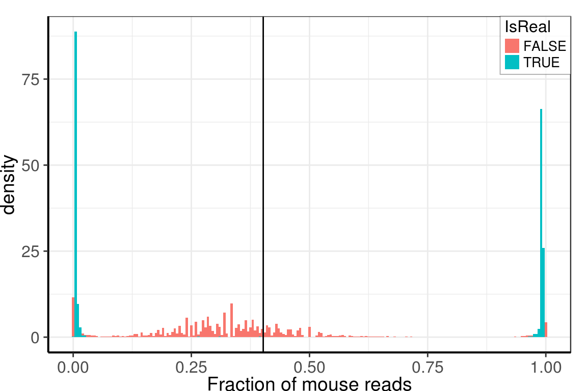
Distribution of total number of molecules by background cells:
gg <- ggplot(umi_by_species %>% filter(!IsReal)) +
  geom_histogram(aes(x=Total), bins=100) +
  scale_x_continuous(limits=c(0, 250), expand=c(0, 0), name="Total #UMIs") +
  scale_y_continuous(limits=c(0,9000), expand=c(0, 0), name="#Cells") +
  theme_pdf()

gg
Session information
data.frame(value=unlist(sessioninfo::platform_info()))| value | |
|---|---|
| version | R version 3.4.1 (2017-06-30) |
| os | Ubuntu 14.04.5 LTS |
| system | x86_64, linux-gnu |
| ui | X11 |
| language | (EN) |
| collate | en_US.UTF-8 |
| tz | America/New_York |
| date | 2018-01-27 |
as.data.frame(sessioninfo::package_info())[c('package', 'loadedversion', 'date', 'source')]| package | loadedversion | date | source | |
|---|---|---|---|---|
| 1 | assertthat | 0.2.0 | 2017-04-11 | CRAN (R 3.4.1) |
| 2 | backports | 1.1.2 | 2017-12-13 | CRAN (R 3.4.1) |
| 4 | bindr | 0.1 | 2016-11-13 | CRAN (R 3.4.1) |
| 5 | bindrcpp | 0.2 | 2017-06-17 | CRAN (R 3.4.1) |
| 6 | clisymbols | 1.2.0 | 2017-05-21 | CRAN (R 3.4.1) |
| 7 | colorspace | 1.3-2 | 2016-12-14 | CRAN (R 3.4.1) |
| 9 | cowplot | 0.9.2 | 2017-12-17 | CRAN (R 3.4.1) |
| 11 | digest | 0.6.14 | 2018-01-14 | cran (@0.6.14) |
| 12 | dplyr | 0.7.4 | 2017-09-28 | CRAN (R 3.4.1) |
| 13 | dropEstAnalysis | 0.6.0 | 2018-01-27 | local (VPetukhov/dropEstAnalysis@NA) |
| 14 | dropestr | 0.6.0 | 2018-01-24 | local (@0.6.0) |
| 15 | evaluate | 0.10.1 | 2017-06-24 | CRAN (R 3.4.1) |
| 16 | ggplot2 | 2.2.1 | 2016-12-30 | CRAN (R 3.4.1) |
| 17 | ggrastr | 0.1.5 | 2017-12-28 | Github (VPetukhov/ggrastr@cc56b45) |
| 18 | git2r | 0.21.0 | 2018-01-04 | cran (@0.21.0) |
| 19 | glue | 1.2.0 | 2017-10-29 | CRAN (R 3.4.1) |
| 23 | gtable | 0.2.0 | 2016-02-26 | CRAN (R 3.4.1) |
| 24 | highr | 0.6 | 2016-05-09 | CRAN (R 3.4.1) |
| 25 | htmltools | 0.3.6 | 2017-04-28 | CRAN (R 3.4.1) |
| 26 | knitr | 1.18 | 2017-12-27 | cran (@1.18) |
| 27 | labeling | 0.3 | 2014-08-23 | CRAN (R 3.4.1) |
| 28 | lattice | 0.20-35 | 2017-03-25 | CRAN (R 3.4.1) |
| 29 | lazyeval | 0.2.1 | 2017-10-29 | CRAN (R 3.4.1) |
| 30 | magrittr | 1.5 | 2014-11-22 | CRAN (R 3.4.1) |
| 31 | Matrix | 1.2-12 | 2017-11-16 | CRAN (R 3.4.1) |
| 33 | munsell | 0.4.3 | 2016-02-13 | CRAN (R 3.4.1) |
| 34 | pkgconfig | 2.0.1 | 2017-03-21 | CRAN (R 3.4.1) |
| 35 | plyr | 1.8.4 | 2016-06-08 | CRAN (R 3.4.1) |
| 36 | R6 | 2.2.2 | 2017-06-17 | CRAN (R 3.4.1) |
| 37 | Rcpp | 0.12.15 | 2018-01-20 | cran (@0.12.15) |
| 38 | rlang | 0.1.4 | 2017-11-05 | CRAN (R 3.4.1) |
| 39 | rmarkdown | 1.8 | 2017-11-17 | CRAN (R 3.4.1) |
| 40 | rprojroot | 1.3-2 | 2018-01-03 | cran (@1.3-2) |
| 41 | scales | 0.5.0 | 2017-08-24 | CRAN (R 3.4.1) |
| 42 | sessioninfo | 1.0.0 | 2017-06-21 | CRAN (R 3.4.1) |
| 44 | stringi | 1.1.6 | 2017-11-17 | CRAN (R 3.4.1) |
| 45 | stringr | 1.2.0 | 2017-02-18 | CRAN (R 3.4.1) |
| 46 | tibble | 1.3.4 | 2017-08-22 | CRAN (R 3.4.1) |
| 49 | withr | 2.1.1 | 2017-12-19 | cran (@2.1.1) |
| 50 | yaml | 2.1.16 | 2017-12-12 | CRAN (R 3.4.1) |
This R Markdown site was created with workflowr